The Science Behind It

How the Calculator Works

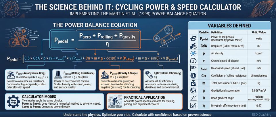
The calculator implements the Martin et al. (1998) power balance equation. In Power to Speed mode, it uses Newton's method to solve for speed numerically. In Speed to Power mode, it computes power directly. Both modes apply the same underlying physics.

The power equation is:

P_pedal = (P_aero + P_rolling + P_gravity) / η

Expanded:

P_pedal = [0.5 × CdA × ρ × (v + v_wind)² × v + Crr × m × g × cos(θ) × v + m × g × sin(θ) × v] / η

Where:

• P_pedal = power at the pedals (watts) - what a power meter measures
• CdA = drag area (m²), the product of drag coefficient and frontal area
• ρ = air density (kg/m³)
• v = ground speed of the bicycle (m/s)
• v_wind = headwind speed (m/s; positive = headwind, negative = tailwind)
• Crr = coefficient of rolling resistance (dimensionless)
• m = total mass of rider + bicycle + gear (kg)
• g = gravitational acceleration (9.8067 m/s²)
• θ = road gradient angle in radians, computed as arctan(gradient% / 100)
• η = drivetrain efficiency (0.97, representing a 3% loss through chain, derailleur, and bottom bracket)

Drivetrain Efficiency

The calculator applies a fixed 3% drivetrain loss. In Power to Speed mode, wheel power is P_wheel = P_pedal × 0.97, and Newton's method solves for the speed at which wheel power equals the sum of aero, rolling, and gravity forces. In Speed to Power mode, total resistive power is divided by 0.97 to give pedal-level power. This matches how a power meter reads: the calculator outputs power at the pedals, not at the wheel.

Wind and Air Speed

The aerodynamic drag force depends on the rider's speed relative to the air mass, not relative to the ground. For a pure headwind or tailwind, that relative speed is (v + v_wind). The drag force is proportional to the square of this air speed, giving the force term 0.5 × CdA × ρ × (v + v_wind)². Power is force multiplied by ground speed, so the full aero power term is 0.5 × CdA × ρ × (v + v_wind)² × v.

This separation of air speed and ground speed is a common error in simplified calculators. The implementation here is correct: the squared term uses air speed (which determines force magnitude), and the final multiplication by v uses ground speed (because power = force × velocity of the application point).

A consequence of this quadratic relationship is that headwinds and tailwinds are asymmetric. Riding into a 15 km/h headwind costs more speed than a 15 km/h tailwind recovers, because drag increases with the square of air speed.

Inputs

Input	Default	Range	Notes
Mode	Power to Speed	-	Switches between solving for speed or for power
Power (W)	-	>0	Used in Power to Speed mode
Target Speed (km/h)	-	>0	Used in Speed to Power mode
Total Weight (kg)	-	40+	Rider + bike + gear combined
Gradient (%)	0	any	Positive = uphill, negative = downhill
CdA (m²)	0.32	0.15-0.50	Drag area; presets for TT/drops/hoods/tops positions
Crr	0.005	0.002-0.015	Rolling resistance; presets for smooth/rough/gravel
Riding Position	Solo	-	Interactive selector: Solo, Wheel (27% drag reduction), Close Draft (35%), Mid-Peloton (50%), Deep Peloton (70%). Applies Blocken et al. drag reduction coefficients to the main speed/power calculation, not just the savings table
Wind Speed (km/h)	0	any	Positive = headwind, negative = tailwind
Air Density (kg/m³)	1.225	0.5-1.5	Auto-calculated from altitude and temperature, or entered manually
Altitude (m)	-	0-5000	Triggers ISA air density calculation
Temperature (C)	-	-20 to 50	Used with altitude for ISA calculation

CdA Position Reference

Position	CdA (m²)
Extreme TT	0.20
TT bike	0.22
Aggressive drops	0.24
Low drops	0.26
Moderate drops	0.28
Standard drops	0.30
Relaxed drops	0.32 (default)
Hoods (aero)	0.34
Hoods (relaxed)	0.36
Tops (tucked)	0.38
Tops (upright)	0.40

Crr Surface Reference

Surface	Crr
Smooth road	0.004
Default	0.005
Rough road	0.006
Gravel	0.008

Air Density: ISA Barometric Formula

When altitude and temperature are provided, the calculator computes air density using the ICAO standard atmosphere barometric formula:

P(h) = P0 × (1 - L×h/T0)^(g×M/(R×L))
ρ    = P(h) / (R_specific × T_actual)

Constants:

• P0 = 101,325 Pa (sea-level pressure)
• T0 = 288.15 K (sea-level standard temperature)
• L = 0.0065 K/m (temperature lapse rate)
• Exponent = g×M/(R×L) = 5.2559 (derived from gravitational acceleration, molar mass of air, and universal gas constant)
• R_specific = 287.058 J/(kg×K)

The actual temperature entered by the user replaces the ISA standard temperature for the density calculation, allowing realistic conditions to be modeled. At sea level (0 m) and 15°C, ρ = 1.225 kg/m³. At 2000 m altitude and 15°C, ρ falls to approximately 1.006 kg/m³, reducing aerodynamic drag by about 18%.

Outputs

Primary Result

• Power to Speed mode: speed in km/h and mph
• Speed to Power mode: required power in watts and W/kg (watts divided by total weight)

Power Breakdown

The calculator shows three components of resistive power:

• Aero: power against aerodynamic drag
• Rolling: power against rolling resistance
• Gravity: power against (or assisted by) gravity; negative on descents

Each is displayed as a watt value and as a percentage of total pedal power. The bar chart shows relative magnitude. On flat road at typical road speeds, aero typically accounts for 70-90% of total resistance.

Time for Common Distances

At the calculated speed, estimated times are shown for: 10 km, 20 km, 40 km TT, 100 km, and 180 km. These assume constant speed and conditions.

Aero Sensitivity Table (Power to Speed mode only)

Shows the effect of changing CdA from 0.20 to 0.40 in steps of 0.02, holding all other inputs constant. Each row shows the resulting speed and the delta from the base CdA. The current CdA row is highlighted. This table quantifies the speed benefit of improving aerodynamic position.

Power Sensitivity Table (Power to Speed mode only)

Shows the speed at 80%, 90%, 100%, 110%, and 120% of the entered power. Each row shows absolute power, the percentage label, resulting speed, and delta from base speed. This table shows the diminishing return on additional power at higher speeds, where aerodynamic drag grows with the cube of velocity.

Drafting Savings Table (Power to Speed mode only, Blocken et al. 2018)

Shows five drafting scenarios based on wheel gap and peloton position. The table reports drag reduction percentage, power saved (watts) to maintain the solo speed, and speed achieved at the original power output with reduced drag:

Position	Drag Reduction	Notes
Solo (no draft)	0%	Baseline
Wheel gap ~2m	27%	Standard following distance
Close draft ~0.5m	35%	Near wheel
Mid-peloton	50%	Sheltered by riders ahead and alongside
Deep in peloton	70%	Well-protected position

Drag reduction is applied as a reduction to CdA: effectiveCdA = CdA × (1 − dragReduction). Power saved is the difference between the original power and the power required to hold the solo speed at the reduced CdA. The speed column shows how fast the rider would travel at the original power with the reduced drag.

In practice, riders typically reduce power when drafting to conserve energy rather than maintaining full power and going faster.

Practical Application

Scenario 1: Flat time trial - "How fast will 250W take me?"

Rider: 75 kg + 8 kg bike = 83 kg total. CdA = 0.27 (aero position). No wind. Flat road. Air density 1.225 kg/m³.

At 250W, solving iteratively: approximately 40 km/h. Aero power dominates, consuming roughly 90% of total power at this speed.

Scenario 2: Hill climb - "What power do I need for a 7% gradient at 15 km/h?"

Same rider, CdA = 0.35 (climbing position).

• Gravity power = 83 × 9.8067 × sin(arctan(0.07)) × 4.17 ≈ 237 W
• Rolling power = 83 × 9.8067 × 0.005 × cos(arctan(0.07)) × 4.17 ≈ 17 W
• Aero power = 0.5 × 0.35 × 1.225 × 4.17² × 4.17 ≈ 6 W
• Total pedal power (divide by 0.97) ≈ 268 W

Gravity accounts for about 88% of total resistance, which is why W/kg drives climbing performance.

Scenario 3: Headwind vs. tailwind asymmetry

250W on a flat road at sea level, CdA = 0.32, mass = 75 kg:

• No wind: approximately 37 km/h
• 15 km/h headwind: noticeably slower (effective air speed rises sharply)
• 15 km/h tailwind: faster, but the gain is smaller than the headwind loss

The asymmetry exists because drag force scales with air speed squared. Equal and opposite winds do not produce equal and opposite speed changes.

The Research

Martin, J. C., Milliken, D. L., Cobb, J. E., McFadden, K. L., & Coggan, A. R. (1998). "Validation of a Mathematical Model for Road Cycling Power." Journal of Applied Biomechanics, 14(3), 276-291.

This study validated cycling power could be predicted from measurable physical parameters with R² = 0.97 and a standard error of 2.7 watts. The researchers validated an SRM power meter against a laboratory ergometer, then measured power during actual road cycling and compared measured values to values predicted by their physics model.

Martin et al. decompose cycling resistance into five forces:

1. Aerodynamic drag - dominant above approximately 20 km/h
2. Rolling resistance - friction between tires and road surface
3. Gravitational resistance - force opposing motion on inclines
4. Wheel bearing friction - minor losses in hubs (omitted in this calculator, absorbed into drivetrain efficiency)
5. Drivetrain losses - energy lost in chain, derailleur, and bottom bracket

Blocken, B., Defraeye, T., Koninckx, E., Carmeliet, J., & Hespel, P. (2018). "CFD simulations of the aerodynamic drag of two drafting cyclists." Computers and Fluids, 71, 435-445.

Blocken et al. used computational fluid dynamics to quantify aerodynamic drag reductions at different wheel gaps and peloton positions. The drafting coefficients in the calculator (27% at ~2m gap, 35% at ~0.5m, 50% mid-peloton, 70% deep in peloton) are drawn from this work.

Limitations

1. Yaw angle is not modeled. The calculator assumes pure headwind or tailwind. Crosswinds alter effective CdA, sometimes reducing drag (sail effect on deep-section wheels) and sometimes increasing it. A complete model would account for yaw-dependent drag.

2. CdA is treated as constant. In practice, CdA varies with speed (clothing flutter changes at higher speeds), with fatigue (riders tend to sit up slightly as they tire), and with yaw angle. The model assumes a single fixed value.

3. Rolling resistance varies with conditions. Crr changes with tire pressure, tire width, surface roughness, temperature, and speed. The default of 0.005 represents a road tire in typical conditions; rough chip-seal or wet roads push Crr toward 0.008 or higher.

4. Altitude: the ISA formula applies to the troposphere. The implementation clamps altitude to 0-11,000 m, which covers the full troposphere. Above 11,000 m the lapse rate changes; this range is irrelevant for cycling.

5. Acceleration is not modeled. The equation solves for steady-state speed only. Repeated accelerations in criteriums, group rides, or hilly courses require additional power for kinetic energy changes. Martin's full model includes this term; the calculator omits it.

6. Bearing friction is omitted. Martin et al. (1998) included a wheel bearing friction term (typically 1-5W). This calculator absorbs that into the 3% drivetrain loss, which is a reasonable simplification for steady-state use.

7. Physiological plausibility advisories. Results requiring sustained power above 6.5 W/kg or producing speeds above 60 km/h on flat terrain trigger informational notes — these levels exceed world-class performance and likely indicate an input error or a non-steady-state scenario.

References

Martin, J. C., Milliken, D. L., Cobb, J. E., McFadden, K. L., & Coggan, A. R. (1998). Validation of a mathematical model for road cycling power. Journal of Applied Biomechanics, 14(3), 276-291. https://doi.org/10.1123/jab.14.3.276

Blocken, B., Defraeye, T., Koninckx, E., Carmeliet, J., & Hespel, P. (2013). CFD simulations of the aerodynamic drag of two drafting cyclists. Computers and Fluids, 71, 435-445. https://doi.org/10.1016/j.compfluid.2012.11.012

Debraux, P., Grappe, F., Manolova, A. V., & Bertucci, W. (2011). Aerodynamic drag in cycling: Methods of assessment. Sports Biomechanics, 10(3), 197-218. https://doi.org/10.1080/14763141.2011.592209

Fintelman, D. M., Sterling, M., Hemida, H., & Li, F. X. (2014). Optimal cycling time trial position models: Aerodynamics versus power output and metabolic energy. Journal of Biomechanics, 47(8), 1894-1898. https://doi.org/10.1016/j.jbiomech.2014.02.029

Grappe, F., Candau, R., Belli, A., & Rouillon, J. D. (1997). Aerodynamic drag in field cycling with special reference to the Obree's position. Ergonomics, 40(12), 1299-1311. https://doi.org/10.1080/001401397187388

Scientific Validation Notes

Power equation is correct. The implementation matches Martin et al. (1998): aerodynamic drag (proportional to air speed squared), rolling resistance (proportional to weight component normal to the road surface), and gravitational resistance (proportional to weight component along the slope). Each force term is multiplied by ground speed v to convert to power.

Drivetrain efficiency is correctly applied. The code divides total resistive power by 0.97 (line 57: (P_aero + P_rolling + P_gravity) / 0.97), and in the speed solver multiplies pedal power by 0.97 to get wheel power before iterating (line 63: P_wheel = power × 0.97). The outputs represent power at the pedals, consistent with how a power meter measures. The earlier article draft incorrectly stated the formula omitted drivetrain efficiency; it does not.

Wind handling is correct. The use of (v + v_wind)² for the drag force term, multiplied by ground speed v for power, matches the physics in Martin et al. This is a common error in simplified calculators; this implementation handles it correctly.

ISA atmosphere model is correctly implemented. The barometric formula with exponent 5.2559 (= g×M/(R×L)) matches the ICAO standard atmosphere specification. Air density is computed from actual user-entered temperature rather than from the ISA temperature profile, which is the appropriate approach for real-condition modeling.

Blocken drafting coefficients are plausible. The drag reductions used (27% at 2m gap, 35% at 0.5m, 50% mid-peloton, 70% deep in peloton) are consistent with the ranges reported in CFD and wind-tunnel studies of cyclist drafting. These values are applied as a reduction to CdA, which correctly scales aero drag while leaving rolling and gravity components unchanged.

Missing terms are minor for steady-state use. Bearing friction and the acceleration/kinetic energy term together account for less than 2% of total power at typical road speeds. Their omission is a reasonable simplification.

Overall: the calculator's core equation is correctly implemented against Martin et al. (1998), drivetrain efficiency is properly accounted for, and the auxiliary models (ISA atmosphere, Blocken drafting) are faithfully represented.